Quickstart

using ActuaryUtilities

cfs = [5, 5, 105]
times    = [1, 2, 3]

discount_rate = 0.03

present_value(discount_rate, cfs, times)           # 105.66
duration(Macaulay(), discount_rate, cfs, times)    #   2.86
duration(discount_rate, cfs, times)                #   2.78
convexity(discount_rate, cfs, times)               #  10.63

10.625805482685935

Features

A collection of common functions/manipulations used in Actuarial Calculations.

Financial Maths

• duration:
  • Calculate the Macaulay, Modified, or signed DV01 durations for a set of cashflows
  • Calculate IR01/CS01 and Effective/Spread risk for curves, contracts, and portfolios
  • Decompose risk by tenor with KeyRates(tenors)
• convexity for price sensitivity
• Flexible interest rate models via the FinanceModels.jl package.
• internal_rate_of_return or irr to calculate the IRR given cashflows (including at timepoints like Excel's XIRR)
• breakeven to calculate the breakeven time for a set of cashflows
• accum_offset to calculate accumulations like survivorship from a mortality vector
• spread will calculate the spread needed between two yield curves to equate a set of cashflows

Key-Rate Sensitivities

Compute key-rate durations, DV01s and convexities for any FinanceModels.jl yield model, without bump-and-reprice. Fixed cashflows use analytic derivatives; valuation callbacks use ForwardDiff.

using ActuaryUtilities, FinanceModels

rates = [0.03, 0.03, 0.03, 0.03, 0.03]
tenors = [1.0, 2.0, 3.0, 4.0, 5.0]
zrc = ZeroRateCurve(rates, tenors)
cfs = [5.0, 5.0, 5.0, 5.0, 105.0]

# Value, key-rate durations, DV01s and convexities in one call
result = sensitivities(SecondOrder(), KeyRates(tenors), zrc, cfs, tenors)
result.value     # present value
result.duration  # key-rate durations (vector)
result.dv01      # key-rate DV01s (vector)
result.convexity # key-rate convexity matrix
result.dollar_convexity # second derivatives without dividing by value

• sensitivities: value, durations and DV01s in one call, and with SecondOrder() convexity and dollar convexity; parallel without KeyRates, per tenor with it
• Dollar risk: duration(DV01(), ...) and convexity(DollarConvexity(), ...) are defined at zero value and add across positions
• Two-curve decomposition: separate IR01 (risk-free) and CS01 (credit spread) sensitivities
• Contracts and portfolios: duration(Effective(), curve, contract; index), Spread(), and sensitivities(curve, contract; index) with the discount and index exposures
• Do-block syntax: custom valuation functions for rate-dependent instruments (callable bonds, floaters, caps/floors)
• Hull–White stochastic model: key-rate sensitivities of Monte Carlo expected values, differentiating through the full simulation pipeline

using FinanceModels: ShortRate
using Random: Xoshiro

hw = ShortRate.HullWhite(0.1, 0.01, zrc)
hw_result = sensitivities(KeyRates(tenors), Scenarios(hw; horizon=6.0, n_scenarios=1000, rng=Xoshiro(42)), cfs, tenors)
hw_result.duration   # key-rate durations under stochastic dynamics

See the Interest-Rate Sensitivities documentation for details.

Risk Measures

• Calculate risk measures for a given vector of risks:
  • CTE for the Conditional Tail Expectation
  • VaR for the percentile/Value at Risk
  • WangTransform for the Wang Transformation
  • ProportionalHazard for proportional hazards
  • DualPower for dual power measure

Insurance mechanics

• policy_duration: the policy duration given an issue date and a date

Typed Rates

• functions which return a rate/yield will return a FinanceCore.Rate object. E.g. irr(cashflows) will return a Rate(0.05,Periodic(1)) instead of just a 0.05 (float64) to convey the compounding frequency. These values are accepted by the supported valuation APIs across the JuliaActuary ecosystem. Use rate(r) when an API needs the scalar value, and preserve the compounding convention separately.

A couple of other notes:

• rate(...) will return the scalar rate value from a Rate struct:

julia> r = Rate(0.05,Periodic(1));

julia> rate(r) ≈ 0.05
true

• You can still pass a simple floating point rate to various methods. E.g. these two are the same (the default compounding convention is periodic once per period):

discount(0.05, 3)

r = Rate(0.05,Periodic(1));
discount(r, 3)

• convert between rates with:

r = Rate(0.05,Periodic(1));

convert(Periodic(2),  r)   # convert to compounded twice per timestep
convert(Continuous(), r)   # convert to continuous compounding

For more on Rates, see FinanceCore.jl. FinanceModels.jl also provides a rich and flexible set of yield models to use.

Documentation

Full documentation is available here.

Examples

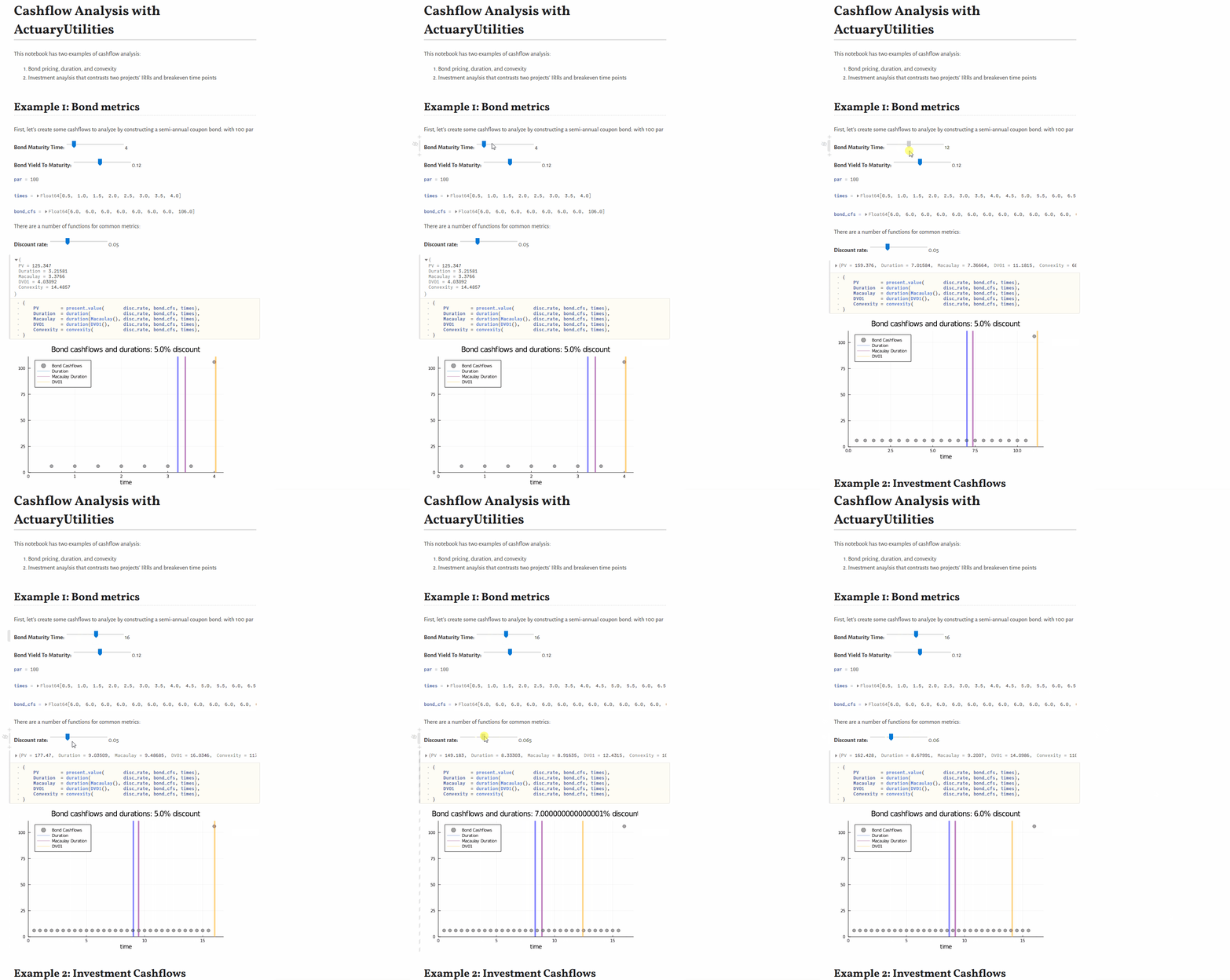
Interactive, basic cashflow analysis

See JuliaActuary.org for instructions on running this example.

Useful tips

Arguments come in this order: a valuation callback (if any), an order marker for sensitivities (FirstOrder() or SecondOrder()), a measure marker such as DV01() or KeyRates(tenors), the rate or curve, then the cashflows and times or a contract. A contract's index curve is the keyword index, which defaults to the curve.